How LLMs Actually Work: A Seven-Layer Map

A seven-layer map of how large language models work, from training data to the app: what's open, what's closed, and which layers builders actually touch.

When a small company starts using AI, the same three questions come up within a week. Should we fine-tune our own model? Should we host it ourselves? Is it safe to send our data to it?

All three are good questions. The trouble is that each one belongs to a different part of the system, and without a map people answer them at the wrong layer. Fine-tuning gets proposed for a problem that retrieval solves in an afternoon. Self-hosting gets proposed to fix a privacy problem that actually lives in the application. "Open source" gets read as "we can see what it was trained on", which is almost never true.

Networking solved this problem decades ago with the OSI model. When I studied for my CCENT, the value of OSI was never the seven boxes themselves. It was that two engineers could say "that's a layer 2 problem" and mean exactly the same thing. LLMs need the same kind of shared vocabulary, and this post is my attempt at one. It comes from building LegalOS, an open-source dialer platform and an agent stack, and from 24 years of running the infrastructure underneath other people's software.

One warning before the map. It is not a clean stack like OSI, and every diagram that pretends it is ends up contradicting itself. Some layers run once, before a model is ever released. Others run on every single message. The first figure shows both.

The map: two flows, seven layers

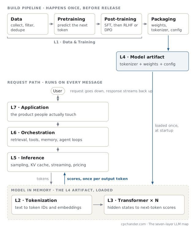Figure 1. The build pipeline runs once and produces an artifact. The request path runs on every message and loads that artifact.

The top half is the build pipeline. Data is collected and cleaned, the model is pretrained, then post-trained into something that follows instructions, then packaged into files. This happens once per model version, at a cost measured in millions of dollars and weeks of GPU time. Unless you work at a model lab, you will never run it.

The bottom half is the request path. A user types into an application (L7). Orchestration code (L6) decides what context and tools to add. An inference server (L5) turns the prompt into tokens and runs the model, producing the answer one token at a time. Inside the model, tokenization (L2) and the transformer (L3) do the actual computation.

The link between the two halves is L4, the model artifact: the files the build pipeline produces and the inference server loads. That is why L4 sits between the two flows in the picture, not in the middle of a stack.

Here are the seven layers, with when each one runs and who usually owns it:

L1 · Data & training. Runs once, before release. Owned by the model lab.
L2 · Tokenization & embeddings. Runs on every request, but was fixed at training time by the lab.
L3 · Transformer. Runs on every request, also fixed at training time.
L4 · Model artifact. The handoff. Owned by the lab, and by you as well if the weights are open.
L5 · Inference & generation. Runs on every request. Owned by an API vendor, or by you if you self-host.
L6 · Orchestration & agents. Runs on every request. Owned by you.
L7 · Application. Runs on every request. Owned by you.

Read the owners from top to bottom. The first four layers are decided before the model reaches you. The last three are where builders actually spend their time, and, not by coincidence, they are also where most of the openness is.

L1 — Data and training: open weights are not open data

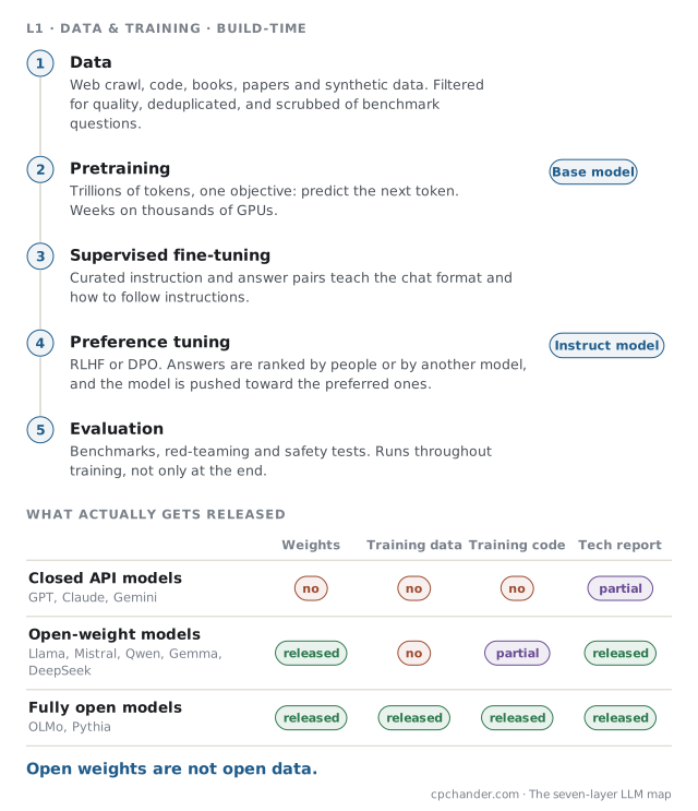Figure 2. Five stages from raw data to an instruct model, and what each kind of model actually releases.

Pretraining is conceptually simple and physically enormous. Take trillions of tokens of text and code, and train the model on a single objective: predict the next token. Llama 3 was pretrained on more than 15 trillion tokens. The result is a base model. It has absorbed a great deal of language and knowledge, but it only knows how to continue text. Ask it a question and it may reply with three more questions, because that is what a list of questions looks like.

Post-training turns that into something useful. Supervised fine-tuning shows the model many thousands of example conversations so it learns the chat format and learns to follow instructions. Preference tuning, through RLHF or the simpler DPO, compares pairs of answers and pushes the model toward the better one. The output is the instruct model, which is the version you actually talk to.

Evaluation is not a step at the end. It runs throughout training: benchmark suites, red-teaming, safety tests, and the internal checks that decide whether an expensive training run is worth continuing.

The table at the bottom of Figure 2 is the most important part of this section. People say "open-source model" and hear "we can inspect how it was made". For almost every model called open, that is false. Llama, Mistral, Qwen, Gemma and DeepSeek release their weights and a technical report. None of them release their training data. Their reports describe the sources in general terms, such as publicly available web data or synthetic data, but you cannot download what actually went in.

Fully open models do exist. AllenAI's OLMo and EleutherAI's Pythia release the weights, the training data, the training code and intermediate checkpoints. Those are the models to reach for if you ever need to audit what a model learned from. For everything else, the accurate term is open-weight. The distinction stops being academic the moment a client asks whether their data could be inside the model, or whether copyrighted material is.

One more thing worth knowing about L1: the good public datasets are much larger than most people expect, and far more heavily filtered. FineWeb, built from Common Crawl, is 15 trillion tokens after deduplication and quality filtering. Most of the engineering in a pretraining dataset is deciding what to throw away.

L2 — Tokenization: the unit you are billed in

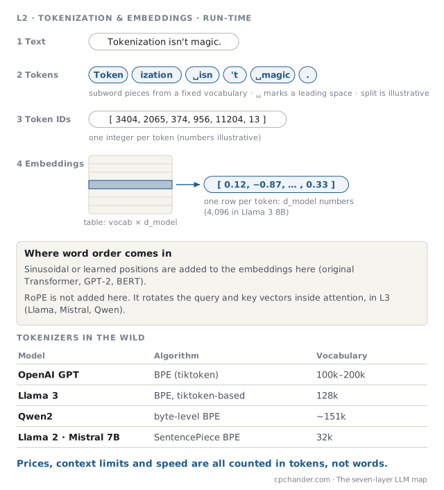Figure 3. Text becomes subword tokens, then integer IDs, then vectors. RoPE, used by most current open models, is not added here.

Models don't read words. A tokenizer splits text into subword pieces drawn from a fixed vocabulary, usually built with byte-pair encoding (BPE). Common words become a single token, and rare words become several. Each token maps to an integer ID, and each ID selects one row of an embedding table, which is a vector of a few thousand numbers. For Llama 3 8B, it is 4,096.

Three practical consequences follow from this.

You pay in tokens, not words. Every API prices input and output per token, and every context window is measured in tokens. A rough rule for English is three to four characters per token. For Hindi and many other languages, the same sentence costs noticeably more tokens, because the vocabulary was built mostly from English text. Budget for that before you launch a multilingual product, not after.

Tokenizers differ, and the details are often wrong in the wild. Llama 3 moved to a 128k-token vocabulary based on OpenAI's tiktoken, while Llama 2 and Mistral 7B used SentencePiece with 32k. Qwen2 uses byte-level BPE with about 151k tokens. A bigger vocabulary means fewer tokens per sentence, at the price of a bigger embedding table.

Word order is handled in two different places. The original Transformer, GPT-2 and BERT add position information to the embeddings, right here in L2. Most current open models instead use RoPE, which rotates the query and key vectors inside attention, in L3. Any diagram that shows position "added to the embeddings" for Llama or Qwen is drawing the older design.

L3 — The transformer: one block, repeated

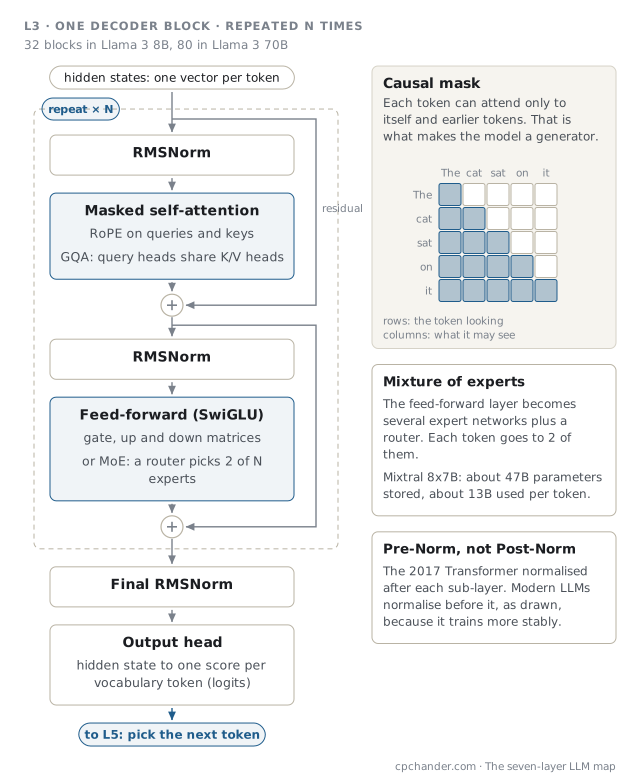Figure 4. A modern decoder block. Llama 3 8B stacks 32 of them; Llama 3 70B stacks 80.

This is the layer every explainer draws, and most of them draw the 2017 version. A modern decoder-only LLM looks like Figure 4:

RMSNorm normalises each token's vector. It is a cheaper variant of LayerNorm (Zhang and Sennrich, 2019), and it comes before each sub-layer. This Pre-Norm arrangement trains more stably than the original Post-Norm.
Masked self-attention lets every token look back at the tokens before it and pull in whatever is relevant. Queries and keys are rotated by RoPE to encode position. Grouped-query attention lets several query heads share one key/value head, which cuts memory use during inference.
A residual connection adds the block's input back to its output, so information and gradients can pass straight through 80 stacked blocks.
A second RMSNorm, then the feed-forward network. Current models use SwiGLU, with three weight matrices (gate, up and down) instead of the two in the original paper.
Another residual add, and then the whole block repeats.

The single most important detail is the causal mask, shown on the right of the figure. When a token computes attention, it may only see itself and the tokens before it. That one constraint is what makes this a generator. During training the model cannot cheat by looking at the word it is supposed to predict, and during inference it builds the answer left to right. A transformer diagram without the mask is describing a different kind of model.

Two variants matter in practice. Mixture of experts replaces the single feed-forward network with several expert networks and a router that sends each token to two of them. Mixtral 8x7B stores about 47B parameters but uses about 13B per token, and DeepSeek-R1 stores 671B and activates 37B. That is how MoE models can be huge on disk and still fast to run. After the last block, a final norm and an output head turn the last token's vector into a score for every token in the vocabulary. Those scores are what L5 works with.

Almost everything in L3 is public: the maths, the papers and the reference implementations. What stays proprietary for closed models is the exact configuration and the trained weights, and those belong to L4.

L4 — The model artifact: it's a folder

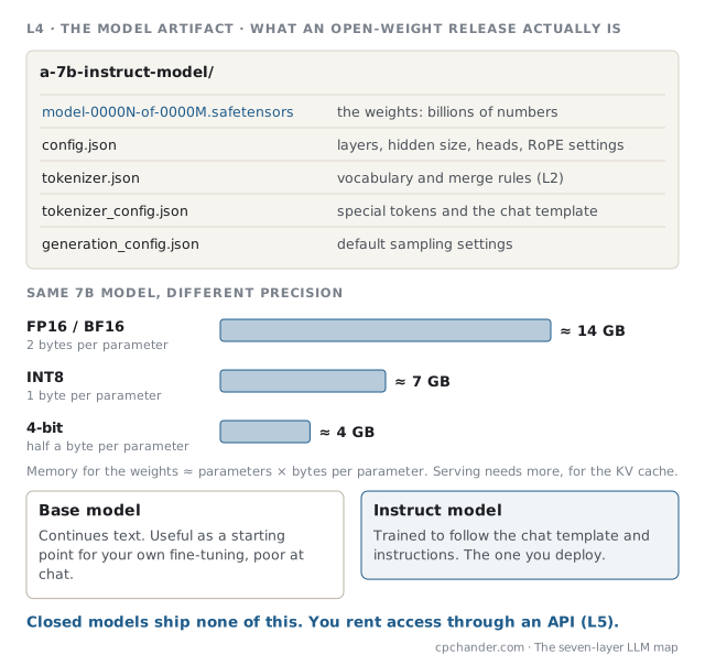Figure 5. What an open-weight release actually contains, and how precision changes its size.

Strip away the branding and an open-weight model is a folder of files. There are the weights, split into safetensors shards. There is a config.json with the architecture numbers: layer count, hidden size, head counts and RoPE settings. There are the tokenizer files, including the chat template, which is the exact text format the model expects for system, user and assistant turns. And there are default generation settings.

Two things in that folder cause most of the confusion I see.

Base versus instruct. Most model families release both. The base model continues text, and the instruct model follows instructions. If someone tells you a model "doesn't follow instructions well", check that they downloaded the right one first. If you plan to fine-tune, the base model is sometimes the better starting point.

Precision decides whether it fits. The memory needed for the weights is the parameter count times the bytes per parameter. A 7B model is about 14 GB at 16-bit, 7 GB at 8-bit and 4 GB at 4-bit. Quantizing to 4-bit costs some quality, usually less than people fear for chat tasks, and it is the reason a 7B or 8B model runs on a laptop through Ollama or llama.cpp. Serving needs more memory than the weights alone because of the KV cache, which is the heart of L5.

Closed models ship none of this. You never see the folder; you rent access to it through an API. That is the real line between open and closed models. It is not the architecture, which is the same transformer either way. It is whether you can hold the artifact.

L5 — Inference: one token at a time

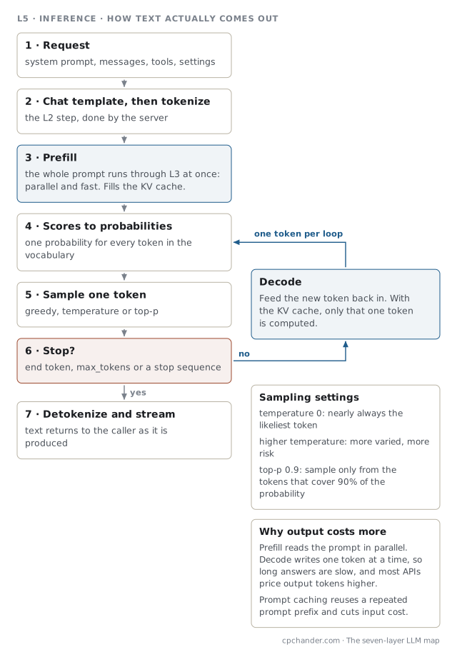Figure 6. Prefill processes the prompt in one parallel pass. Decode then produces the answer one token per loop.

This is the layer almost every diagram skips, and it explains most of what users actually notice: speed, cost and randomness.

When a request arrives, the server applies the chat template and tokenizes the prompt. Then comes prefill: the whole prompt runs through the transformer in one parallel pass. Along the way, the model stores each token's key and value vectors in the KV cache. Prefill is quick because it is parallel, so a long prompt costs compute but not much waiting.

Then the loop begins. The output head produces a probability for every token in the vocabulary, and the server samples one. Greedy decoding picks the most likely token. Temperature flattens or sharpens the distribution. Top-p limits the choice to the likeliest tokens that together cover, say, 90% of the probability. The chosen token is fed back in, which is the decode step, and because of the KV cache only that one new token has to be computed. This repeats until the model emits an end token, reaches max_tokens, or produces a stop sequence. Then the tokens are converted back to text and streamed to the caller.

Once you see the loop, a lot of behaviour stops being mysterious:

Output is slower and more expensive than input. Input is processed in parallel, and output is produced one token at a time. Most APIs price output tokens several times higher than input tokens.
Long conversations get expensive, because the whole history is sent again as input on every turn. Prompt caching reuses a repeated prefix, such as a long system prompt or a reference document, and cuts that cost sharply.
The same prompt can give different answers, because of sampling. Temperature 0 makes the output close to repeatable, but not guaranteed.
Serving memory grows with context length times concurrent users, because every active conversation holds its own KV cache. vLLM's PagedAttention exists to manage exactly that.

This is also where tool calls happen. Instead of text, a model can emit a structured tool call: a tool name and JSON arguments. The model does not run the tool. Your code does. That handoff is where L6 begins.

In practice there are four ways to run L5: a hosted API; an open model on a cloud GPU using vLLM; a local runtime such as Ollama or LM Studio; or a gateway such as LiteLLM or OpenRouter in front of several of them. All four appear in my own working stack, each for a different job.

L6 — Orchestration: a model in a loop

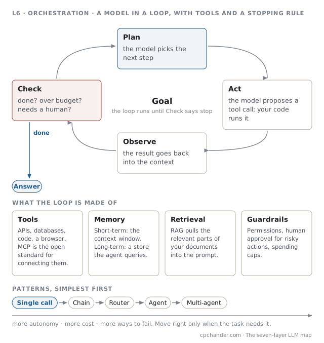Figure 7. An agent is a model in a loop, with tools and a stopping rule.

Most of the "AI" in a real product lives here, and it is written in ordinary code. Orchestration decides what goes into each request and what happens to each response: which documents to retrieve, which tools to offer, what to remember, and when to stop.

An agent is this layer running in a loop. In the plan step, the model picks the next step. In the act step, it proposes a tool call and your code executes it. In the observe step, the result goes back into the context. In the check step, the code asks whether the task is done, over budget, or at a point that needs a human. The loop runs until the check says stop.

The loop is built from four kinds of parts:

Tools: APIs, databases, code execution and browsers. The Model Context Protocol has become the open standard for connecting tools to models, so a tool written once works across many models and clients. The SDR agent I'm building is MCP-based.
Memory: short-term memory is simply the context window. Long-term memory is a store the agent queries, such as a database, a vector index or a notes file.
Retrieval: RAG, covered in the next section.
Guardrails: permissions on which tools may run unattended, human approval for anything that sends, pays or deletes, and hard spending caps.

The most useful rule I know for this layer is to start with the simplest pattern that works. A single call beats a chain. A chain beats a router. A router beats a free-running agent, and one agent beats several. Every step toward autonomy adds cost and new ways to fail: loops that never end, the wrong tool chosen with confidence, a bill that spikes overnight. Move toward autonomy only when the task demands it, and put tracing in first. That means logging every prompt, tool call, result, token count and latency, for every step.

RAG or LoRA: two ways to make a model yours

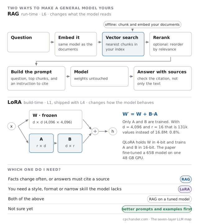Figure 8. RAG changes what the model reads at run time. LoRA changes how it behaves, and is trained once.

"Should we fine-tune?" is usually the wrong first question. There are two main ways to make a general model work for your business, and they live in different layers.

Retrieval-augmented generation (Lewis et al., 2020) runs in L6, on every request. Your documents are split into chunks and embedded ahead of time into a vector index. When a question arrives, it is embedded too, the nearest chunks are found and optionally reranked, and they are pasted into the prompt with an instruction to cite them. The model's weights never change. RAG is the right tool when facts change often, when answers must cite a source, or when the data is private and must stay out of any training run.

LegalOS is built on this pattern. Advocates ask questions of a case file, and every answer cites the page it came from. Embeddings and OCR run locally, so case documents never leave the server, and a four-tier answer cache keeps the cost of repeat questions near zero. Look at that feature list and almost none of it is the model. It is OCR, chunking, retrieval, citations and caching, which is to say it is L6 and L7.

LoRA (Hu et al., 2021) works in L1 and ships with L4. It freezes the model's weight matrix W and trains two small matrices, A and B, whose product is added to it. For a matrix 4,096 wide with a rank of 16, you train about 131 thousand values instead of 16.8 million, which is under 1%. QLoRA goes further by holding the frozen weights in 4-bit; the paper fine-tuned a 65B model on a single 48 GB GPU. LoRA is the right tool for a style, a format or a narrow skill the base model lacks. It is a poor way to teach facts, because those facts go stale and the model cannot cite where it learned them.

The decision in practice:

If facts change often, or answers must cite a source, use RAG.
If you need a style, a format or a narrow skill, use LoRA.
If you need both, run RAG on top of a tuned model.
If you're not sure yet, write better prompts with a few worked examples first. It is the cheapest option, and it solves more than people expect.

L7 — Application: the model is a component

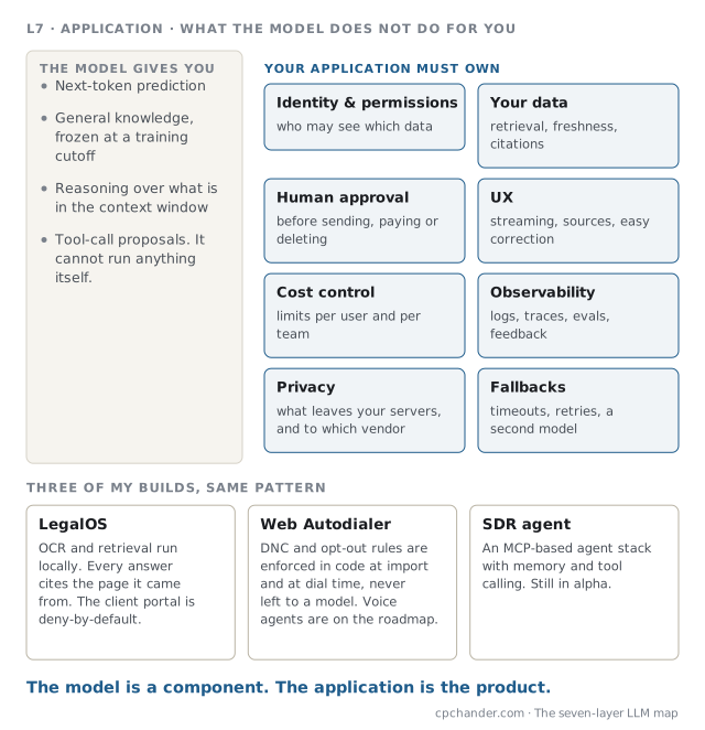Figure 9. What the model provides, and everything the application still has to own.

The model gives you next-token prediction, general knowledge frozen at a training cutoff, reasoning over whatever is in the context window, and tool-call proposals. That is all it gives you. Everything a business actually needs from an AI product sits in L7.

Start with identity and permissions. The model has no idea who is asking, so your application must make sure retrieval only returns what that particular user is allowed to see. I wrote about enforcing that at the database level for a multi-tenant HRMS, and the same row-level thinking applies to a vector index. Then come human approval before anything irreversible, and a UX that streams, shows sources and makes correction easy. Then cost limits per user and per team; logs, traces, evals and a feedback button; a clear answer to what data leaves your servers and which vendor receives it; and fallbacks for when the model times out or refuses.

On the Web Autodialer, DNC and opt-out rules are enforced in code, once at import time and again at dial time. Voice agents are on that platform's roadmap, and the principle holds regardless: a compliance rule is not something to leave to a model's judgment, however good the model gets.

Five things most LLM diagrams get wrong

Most one-page LLM diagrams I've seen, including the first drafts of these, share the same five mistakes. They are worth knowing because each one leads to a bad decision.

They draw a single stack. Training and serving are separate flows that meet at the artifact. A single stack forces contradictions: is the model "below" the transformer, or made of it?
They call open-weight models open-source and imply open data. The weights are released; the data almost never is.
They draw the 2017 transformer. That means Post-Norm, no causal mask, positions added to the embeddings and a two-matrix feed-forward layer. Modern models differ on all four.
They skip generation. Without the prefill and decode loop, you cannot explain why output costs more, why answers vary, or why long chats get expensive.
They stop at the model. The layers where builders spend their time, orchestration and the application, get a single box labelled "apps".

What I'd tell a small company starting today

Start at L7 and work down, not the other way round. Write down the job the tool must do, who is allowed to see what, and which actions need a human to approve them. Then choose the L6 pattern, which is usually a single call or a short chain with retrieval. Then pick a model through an API, behind a gateway so you can swap it later. Only go down to L4, meaning open weights and self-hosting, when you have a specific reason: data that cannot leave your servers, very high volume, offline use, or a fine-tuned model you need to own outright. Almost nobody needs to touch L1.

Two habits are worth setting on the first day. Put tracing and cost tracking in before the first user arrives, not after the first surprising invoice. And write evals, a fixed set of questions with known good answers, before you tune a single prompt. That turns "it feels better" into a number you can compare.

I made a related argument in my read of Arvind Narayanan's "AI as Normal Technology": capability arrives fast, and the value comes from the unglamorous integration work around it. This map is the same point, drawn out. Four layers are decided before the model reaches you. Three are yours, and that is where the work is and where the advantage is.